Calculated items in OBIEE Pivot tables can be very useful in certain reporting circumstances, either for ease of development, or to meet specific report requirements. While calculated items in OBIEE are easy, and flexible, they do have one important drawback: they take on the data and display formatting of the fact column they are calculated against.
The most common case is the calculation of a % change across a time dimension in financial reporting ( Year over Year, Quarter over Quarter, etc.). 1 This type of calculation usually takes the form of a percent change calculation similar to below:
(( $2 - $1 ) / $1) *100
By default, if you perform this calculation against a numerical fact ( sales, customers) you will run into the problem of how to display the % change in the correct format, since the calculated % will want to take the form of the fact it is calculated against, as can be seen in the example 2 below:
 |
| Figure 1 - Pivot Table |
 |
| Figure 2 - Calculated item |
 |
Figure 3 - Results
|
Not very pretty at all.
- Use HTML formatting tricks to “hide” trigger text in the results, then conditionally format off those triggers. While inventive, as the comments note, this solution falls flat if the report is ever printed, as the PDF engine will pick up and display all of the hidden characters.
- Convert the pivot table to a regular table with some complex column formulas. Very time consuming and cumbersome, would also not solve the requirement of showing the dimension values noted as noted in Footnote1.
- Convert the calculated result to text and manually add your formatting characters. I don’t think this actually works since the calculated fields won’t accept logical SQL functions, and this would be very cumbersome.
- Add a column that is a COUNT DISTINCT on the dimension that you are calculating across ( in the displayed example, “Time T05 Per Name Year”. This column will serve as your “trigger” to apply your conditional formatting.
 Figure 4 - Column Formula
- For each of your facts, apply a conditional format that is triggered when the above column value is zero. In the formatting, apply whatever visual and data formats you desire. In this example we will format the data as a percent, with one decimal place.
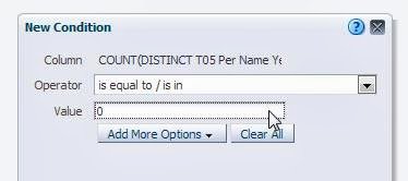
Figure 5 - Condition

Figure 6 - Format when condition is met
- Exclude the “trigger” column from your pivot view. View your results and be satisfied:

Figure 7 - Correct formatting of calculated item.
* Note that this would also allow you to apply visual formatting if you wanted to distinguish this row/column as a total.
Why it works
The use of conditional formatting that applies a data type as part of the format is a straightforward leap of logic, but what to use as the trigger? Most people will try to use the dimension they have setup the calculation in. However, if you try to use the text description given to the calculated item you will find that the condition is never applied: |
| Figure 8 - Condition on dimension |
 |
| Figure 9 - Condition never met, format never applied |
If you try to setup a filter that is true when the dimension is not in reasonable range of values ( in this example we try to format off all years not in the 2000s ) you will find that your calculated item is skipped as well (this has the added vulnerability of being very explicit):
 |
| Figure 10 - Condition on dimension values |
 |
| Figure 11- Condition never met, format never applied |
The reason for all this is that the calculated item “borrows” EACH of the dimension values it operates against. Hence, no matter how inventive your filter is, as long as you are trying to somehow separate the calculated member away from the members it is operating on, you will never succeed. This member “borrowing” is apparent if you add the dimension it operates against to the query a 2nd time, and look at the table view.
 |
| Figure 12 - Calculated item "borrows" members |
But since the “member value” given to the calculated item does not actually exist in the dimension, if you try to perform a count distinct against it, you will always get zero.
 |
| Figure 13 - Count distinct against dimension |
There is your difference; there is your “trigger.” The rest is basic formatting.
1: You might suggest that this requirement is better served using column(s) with time series calculations, and you might be right. However, more often than not the user will want to SEE the time periods being compared ( 2012 vs 2011, or 08/07/2012 vs 08/07/2011). When using facts with time series calculations you will only be able to show “this year” vs “last year” since the column heading of the time series calculated fact will always be static. In these cases you will need to use the base fact and a time dimension, along with the solution provided here.
2: All screen shots, and examples used in this post are performed in Sample App V305. An XML of the final correctly formatted report can be downloaded here.
17 comments:
I wonder why...
After spending $$$$$$ on a "Cutting Edge" BI Suite...I wonder why such usability issues have not been addressed. Why does one need to "hack" using html/javascript or spend enormous amounts of time trying to find "workaround" to seemingly simple usecases?
I agree with you completely, If we are able to set the visual style of the calculated member heading, why not the data itself as well? Spending time doing these types of things is not value-add. But is is necessary, as presentation is as important as the data itself.
On the other hand the ability to "hack" to expand the capabilities of the tool using java / css / html is completely value-add.
I'm trying this out but it's not working for my total/grand total percent change. The conditional formatting doesn't work on the total. I'm probably missing something obvious but I really don't find any of this very obvious.
Hey John,
I see what you are saying. You're not missing anything obvious, it appears the grand total row ALWAYS takes the data format form of the base fact column, and there is no way to override this. I tried editing the XML to force the conditional format rule into the grand total column, and though I can get the UI to accept the edited XML, it throws an error when i try to run the report.
I will continue to work with it, but as of now the lack of work around for the grand total row is still a considerable limitation.
Really helpful post this - thanks.
However, this all works perfectly until I drag the "trigger" column to Exclude, and then I get an error:
View Display Error. Error getting cursor in GenerateHead.
Any ideas why this might be happening?
The measure column references the "trigger" column via a column reference expression in the XML.
I suspect when you exclude the trigger column the measure column can no longer "find" the trigger column via reference.
Leave the trigger column as a hidden dimension in your pivot table if possible. If that is not possible then you may have to edit the XML to get the measure column to format off of a "hidden" SQL expression. I wee see if I can duplicate this behavior in my test environment and post up steps to resolve.
Ah, OK, I'd been getting the count distinct metric by duplicating the layer in my measures section, and these cannot be hidden. OK, I'll see if I can create a separate count distinct column.
Thanks for your help!
I was unable to reproduce this error on the Sample app environment and was scratching my head, but now I see that you are duplicating the column in the pivot table.
Create a stand alone column and you should be able to exclude it from your query.
Hi Victor,
I've achieved the same result by directly testing the base fact column (the year in your example) for "IS NULL". If you replace the total line with another calculated item that sums the row categories, the conditional format will work.
Jerry C.
Jerry, I like the IS NULL solution. It prevents the need to create the calculated column. Can you point me in a direction to know how to do the calculated item that sums the rows instead of using the pivot table grand total?
What if more than two calculated itoms one is percentage and the other is number. this will result all the calculated items %
@ Jerry,
just tried to test "is null" on the base dimension today and it did not work. I had to create the calculated column again.
I find that does not work when using variables in the calculated item (such as $1, $2, etc). It does work if I use the member values (but of course, using the measure values is no help and makes the report unusable).
Jayaprakash,
I created an additional "+/- Difference" calculated item, $2 - $1 and changed my trigger column to
COUNT(distinct "Time."T05 Per Name Year") + RCOUNT("Time."T05 Per Name Year" BY)
this results in:
2012 = 3
2011 = 2
+/- Difference = 1
YOY = 50
conditionally format using constants 1 and 50 accordingly
hope this helps
Anybody worked out the formatting on the grand total column yet?
Hello, How do you create a calculated item in a pivot that is reading from a direct database request?
Post a Comment